摘要
Tacotron2:Tacotron 的改良版。Tacotron应该是第一个基于深度学习的端到端语音合成模型。
论文及代码
论文
Natural TTS Synthesis By Conditioning Wavenet On Mel Spectrogram Predictions
代码
https://github.com/NVIDIA/tacotron2
详细介绍
模型
由Encoder、Location Sensitive Attention 和 Decoder、PostNet组成,解码器是WaveNet。
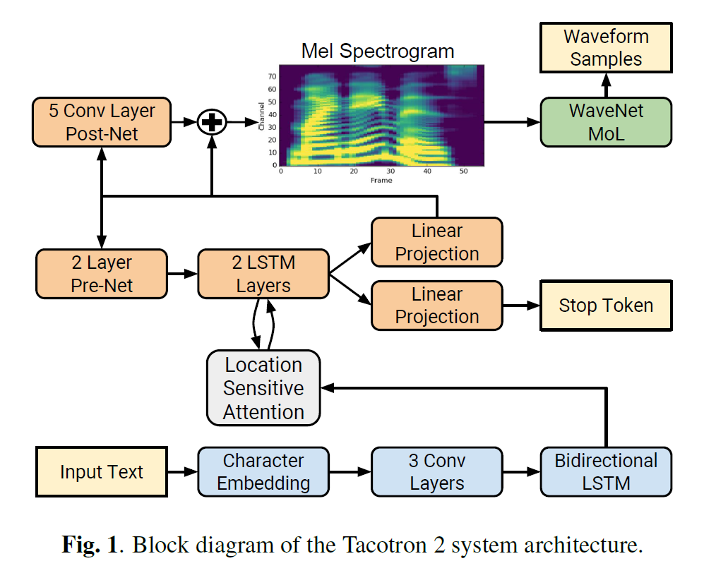
Encoder
由 Character Embedding、3个一维卷积和一个双向LSTM组成。
- Character Embedding:将 text-index 映射到 [1, 512]维;
1
2
| 维数变化:[32, 161] ----> [32, 512, 161], 32为batch_size的大小,161为当前batch_size下最长的句子的音素长度
nn.Embedding(hparams.n_symbols, hparams.symbols_embedding_dim)
|
- 一维卷积:主要是由于实践中RNN很难捕获长时依赖,这里使用卷积层获取上下文;
1
2
3
4
5
6
7
8
9
10
11
12
| 维数变化:[32, 512, 161] -----> [32, 512, 161]
convolutions = []
for _ in range(hparams.encoder_n_convolutions):
conv_layer = nn.Sequential(
ConvNorm(hparams.encoder_embedding_dim,
hparams.encoder_embedding_dim,
kernel_size=hparams.encoder_kernel_size, stride=1,
padding=int((hparams.encoder_kernel_size - 1) / 2),
dilation=1, w_init_gain='relu'),
nn.BatchNorm1d(hparams.encoder_embedding_dim))
convolutions.append(conv_layer)
self.convolutions = nn.ModuleList(convolutions)
|
1
2
| 维数变化:[32, 512, 161] -----> [32, 161, 512]
x = x.transpose(1, 2)
|
- 双向LSTM(隐藏层是256,由于是双向LSTM,最总结果是256维concat256维,最终就是512维):
1
2
3
4
| 维数变化:[32, 161, 512] -----> [32, 161, 512]
self.lstm = nn.LSTM(hparams.encoder_embedding_dim,
int(hparams.encoder_embedding_dim / 2), 1,
batch_first=True, bidirectional=True)
|
Encoder 将字符映射到了一个512维的隐状态。
Location Sensitive Attention 和 Decoder
代码中将 Attention与Decoder放到了一起,这里就放到一起解释。
训练阶段用到Teacher Forcing。
1
2
3
4
5
6
7
8
9
10
| self.n_mel_channels = hparams.n_mel_channels # 80 mel 通道数
self.n_frames_per_step = hparams.n_frames_per_step # 1 每次预测1帧
self.encoder_embedding_dim = hparams.encoder_embedding_dim # 512 隐层维数
self.attention_rnn_dim = hparams.attention_rnn_dim # 1024 attention维数
self.decoder_rnn_dim = hparams.decoder_rnn_dim # 1024 decoder维数
self.prenet_dim = hparams.prenet_dim # 256 prenet维数
self.max_decoder_steps = hparams.max_decoder_steps # 1000 预测最大1000步
self.gate_threshold = hparams.gate_threshold # 0.5 Stop Token的概率
self.p_attention_dropout = hparams.p_attention_dropout # 0.1 dropout
self.p_decoder_dropout = hparams.p_decoder_dropout # 0.1 dropout
|
1
2
3
| memory:encoder_output, encoder 的输出,维数为[32, 161, 512]
decoder_input:初始输入[1, 32, 80],全为0的向量
decoder_inputs:真实mel谱[32, 80, 886]
|
1
2
| 维数变化:[32, 80, 886] -----> [886, 32, 80]
解析decoder_inputs
|
- cat decoder_input and decoder_inputs
1
| 维数变化:[32, 80, 886] -----> [886, 32, 80]
|
- Prenet:作为一个信息瓶颈层(boottleneck),对于学习注意力是必须的
1
2
3
4
5
6
7
8
9
| 维数变化:[887, 32, 80] -----> [887, 32, 256]
self.prenet = Prenet(
hparams.n_mel_channels * hparams.n_frames_per_step,
[hparams.prenet_dim, hparams.prenet_dim])
# Prenet:两个线性层
in_sizes = [in_dim] + sizes[:-1]
self.layers = nn.ModuleList(
[LinearNorm(in_size, out_size, bias=False)
for (in_size, out_size) in zip(in_sizes, sizes)])
|
1
2
3
4
5
6
7
8
9
10
11
12
13
14
15
16
17
18
19
20
21
22
23
24
25
26
27
28
| # B 为 batch_size 32
# MAX_TIME 为 当前 batch 中句子最长的长度 161
self.attention_hidden = Variable(memory.data.new(
B, self.attention_rnn_dim).zero_()) 维数:[32, 1024]
self.attention_cell = Variable(memory.data.new(
B, self.attention_rnn_dim).zero_()) 维数:[32, 1024]
self.decoder_hidden = Variable(memory.data.new(
B, self.decoder_rnn_dim).zero_()) 维数:[32, 1024]
self.decoder_cell = Variable(memory.data.new(
B, self.decoder_rnn_dim).zero_()) 维数:[32, 1024]
self.attention_weights = Variable(memory.data.new(
B, MAX_TIME).zero_()) 维数:[32, 161]
self.attention_weights_cum = Variable(memory.data.new(
B, MAX_TIME).zero_()) 维数:[32, 161]
self.attention_context = Variable(memory.data.new(
B, self.encoder_embedding_dim).zero_()) 维数:[32, 512]
self.memory = memory 维数:[32, 161, 512]
# memory 是 encoder 的 outputs, 维数是 512 维
# processed_memory 是这样处理的:将 512 维 映射到 128 维,同时激活函数是 tanh,结果是 [-1, 1]
self.processed_memory = self.attention_layer.memory_layer(memory) 维数:[32, 161, 128]
|
- decode (attention and decode)
| 应该是最核心关键的部分了
接下来利用 teacher forcing 生成 mel 谱,空的数组生成第一帧 mel,真实的第一帧mel生成第二帧mel,以此类推
- 第一层 LSTM:
LSTM 的 前向传播 ht, Ct = Lstmcell(xt, h(t−1), C(t−1))
1
2
3
4
5
6
| # 第一帧 mel:decode_input,维数[32, 256]
cell_input = torch.cat((decoder_input, self.attention_context), -1) # 这个就相当于 x_t
self.attention_hidden, self.attention_cell = self. attention_rnn(
cell_input, (self.attention_hidden, self.attention_cell))
|
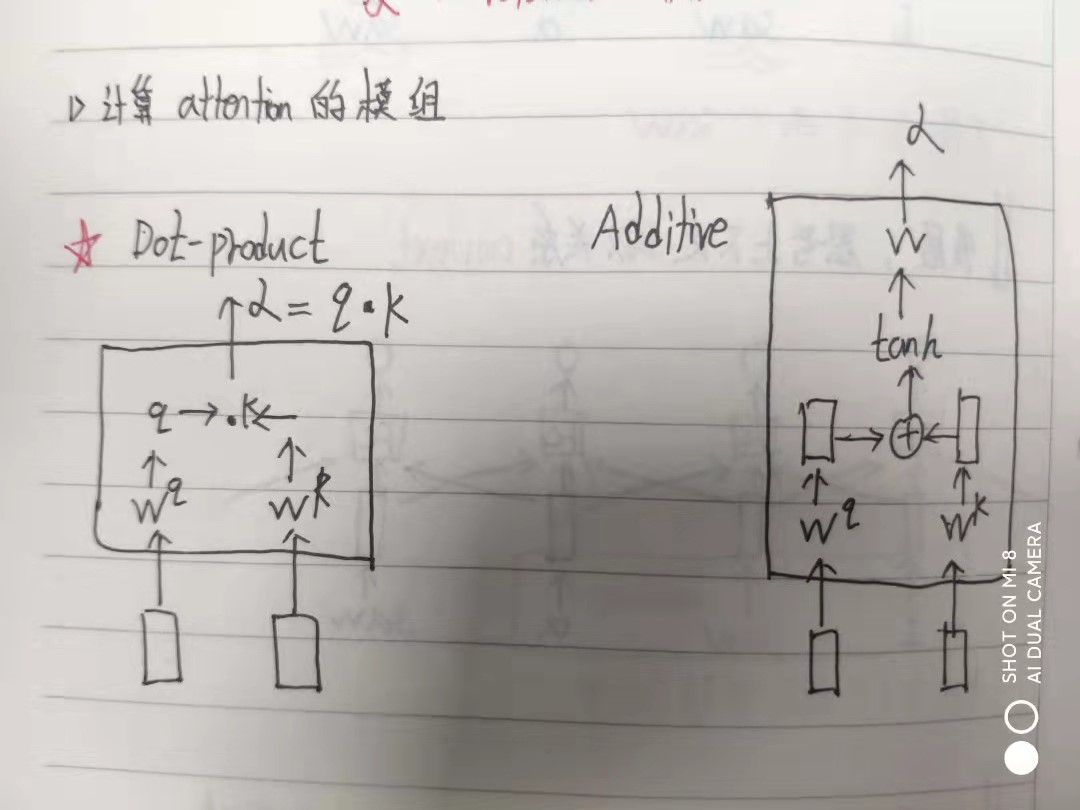
| 这里要介绍两个注意力机制:Dot-product (这个是self-attention论文里用到) 和 Additive(这个是Tacotron2用到的)。详细看图片
- 内容注意力:
利用 1. 中获得的 attention_hidden 计算 Q
1
2
3
4
5
6
| # 维数变化:[32, 1024] -----> [32, 1, 128]
self.query_layer = LinearNorm(attention_rnn_dim, attention_dim,
bias=False, w_init_gain='tanh')
# 1024 --> 128 , 同时利用 tanh 将结果映射到 [-1, 1]
processed_query = self.query_layer(query.unsqueeze(1)) # 这里query就是 self.attention_hidden
|
- 位置注意力:
位置注意力就是基于 attention_weights 的,这里不包含内容信息
1
2
3
4
5
6
7
8
9
10
11
12
13
14
15
| # 输入
attention_weights_cat = torch.cat(
(self.attention_weights.unsqueeze(1),
self.attention_weights_cum.unsqueeze(1)), dim=1) 维数:[32, 2, 161]
# 网络
padding = int((attention_kernel_size - 1) / 2)
self.location_conv = ConvNorm(2, attention_n_filters,
kernel_size=attention_kernel_size,
padding=padding, bias=False, stride=1,
dilation=1) 一维卷积
self.location_dense = LinearNorm(attention_n_filters, attention_dim,
bias=False, w_init_gain='tanh') 线性层
维数变化 [32, 2, 161] -----> [32, 161, 128]
|
- 计算 Attention
将 processed_memory 与 2. 计算的 Q 与 3.计算的 L 相加,计算最终 Attention
1
2
3
4
5
| energies = self.v(torch.tanh(
processed_query + processed_attention_weights + processed_memory))
# energies 与 alignment 是一个东东
attention_weights = F.softmax(alignment, dim=1) # 将权重映射到 【0, 1】
维数变化: [32, 161, 128] -----> [32, 161, 1] -----> [32, 161]
|
- 计算 attention_context
1
2
3
4
5
6
| attention_context = torch.bmm(attention_weights.unsqueeze(1), memory)
# print(memory.shape)
# torch.bmm 矩阵乘法
# (32 * 1 * 161) %*% (32 * 161 * 512)
attention_context = attention_context.squeeze(1)
# 32 * 512
|
- 第二层LSTM
1
2
3
4
5
6
7
8
9
10
11
12
13
14
15
16
17
18
| # 预测 mel 谱,及Stop Token
decoder_input = torch.cat(
(self.attention_hidden, self.attention_context), -1) # 上一层LSTM返回的hidden与 5. 计算的attention_context
self.decoder_hidden, self.decoder_cell = self.decoder_rnn(
decoder_input, (self.decoder_hidden, self.decoder_cell)) #
self.decoder_hidden = F.dropout(
self.decoder_hidden, self.p_decoder_dropout, self.training)
decoder_hidden_attention_context = torch.cat(
(self.decoder_hidden, self.attention_context), dim=1)
decoder_output = self.linear_projection(
decoder_hidden_attention_context) # 32 * 80
gate_prediction = self.gate_layer(decoder_hidden_attention_context) # 32 * 1
|
接下来while循环所有帧!
Post-Net
Five 1-d convolution with 512 channels and kernel size 5. 精调 decoder 获得的Mel谱!
Inference
- 利用上一帧预测的mel作为输入,而不是真实的mel;
- Dropout 在推断阶段也是 true!
绘制对齐图与MEL谱图
Tacotron2绘制的 mel 图是真的漂亮,这里扒一下代码,为后续准备。
1
2
3
4
5
6
| path = "BZNSYP-mel-000001.npy"
a = np.load(path)
fig, ax = plt.subplots(figsize=(6, 3))
ax.imshow(a.T, aspect="auto", origin="lower",
interpolation='none')
这里保存的 .npy 文件是 Tacotron2 中STFT获得的 mel 谱
|